


Category: General
Sep 21, 2022
A Simple Explanation of Neural Networks for Business People
Introduction
Nobel Laureate Richard Feynman said, “When we speak without jargon, it frees us from hiding behind knowledge we don’t have. Big words and fluffy business-speak cripple us from getting to the point and passing knowledge to others.”
A grasp of the fundamentals of AI Neural networks can be useful to most business executives; however, artificial intelligence articles often require a reasonable understanding of advanced math. They invariably start by comparing neural networks and the brain’s workings. This article will explain specifically feed-forward neural networks without using either.
If you have any previous learning on AI, I am confident you have seen some form of the following diagram. It represents a small, simple, fully connected, deep neural network.
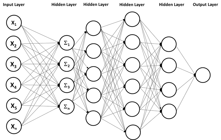
Note — A network of this small is not likely. The same outcome can be derived from simpler forms of machine learning.
But what does this network do? It simply produces mathematical functions for lines, planes, or shapes that separate or group data. That is it. That is the function of a neural network. Admittedly the shapes created by a typical neural network are multidimensional and impossible to conceptualize for all but the most brilliant people.
This example shows a plot of two things, Thing One in Purple and Thing Two in Green, and a line that separates them into groups.
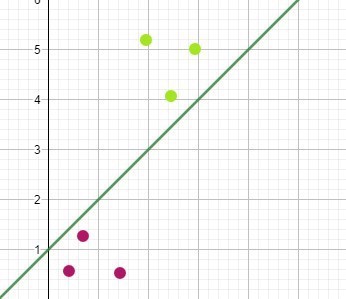
A neural network is conceptually learning the mathematical function for that line. Once the network model has “learned” the math function for the line, a user can input information about a thing, i.e., the coordinates. The system will output the classification; these coordinates are to the right of the line; therefore, they represent Thing One.
A neural network connects input (features) and output (labels). Suppose I am trying to differentiate between Oranges and Bananas from features alone. The input might be the color of an object, and the output is the label Banana or Orange, both in numerical form.
The network learns the mathematical functions for lines or shapes that separate the data (this is a cat, this a dog) or fits the data (I predict this house’s price is $100k). A neural network performs multiplication, addition, and transformations to millions of numbers, each time changing its initial guess to improve the model’s accuracy. The objective of the training process is to find the numbers (called weights and biases) that result in a minor difference between the outputs of the network and the known truth.
The training process digests many examples of data relationships. The training data consists of the answer and the input features related to that answer. There are two labels in the following training data example (Car, Motorcycle) and three features (Height, Length, Weight).
Note — The choice of features here is poor and would result in a flawed AI model.
How Does it Work?
The neural network diagram in the introduction may look complicated, but it is simply a collection of smaller building blocks that look like this:

A single input feature is represented by X1. The weight is represented by W1. The strange “E” shape is the sum of the input multiplied by the weight. The B is an additional value called a Bias that is added to the previous sum. The result, called a weighted sum, is from the following mathematical function,
Weighted Sum =X1*W1+B
This is the core function of every neural network.
Note — Before being passed as an output, the weighted sum undergoes a transformation using an activation function. The activation function changes one number to another number. In simple terms, the activation function changes a linear output to a non-linear output or a straight line into a curved line.
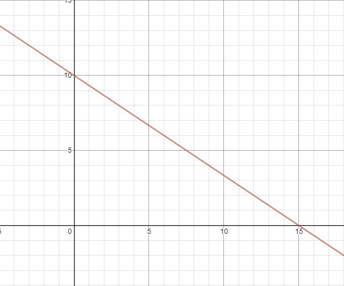
Changing the letters from the earlier diagram and examining it more closely, you will recognize that this is the function for a straight line, i.e., Weighted Sum = X1*W1+B is the same as Y=MX+C, where M is the slope of the line and C is the slope-intercept of the Y-axis. The single neuron represents a linear function.
Now, look at this expanded neural network.
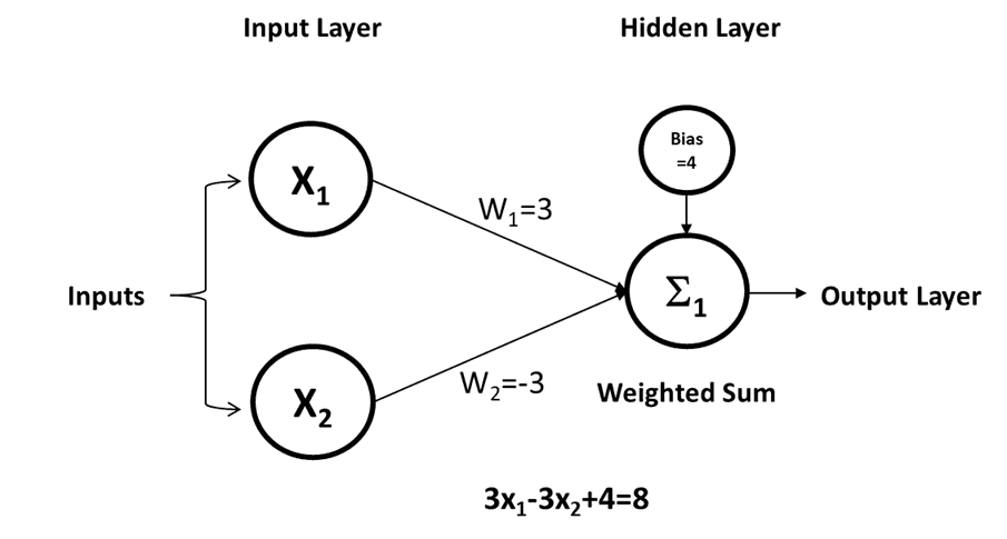
It takes two inputs instead of one, and if you examine each input individually, you will see that the resulting function is
Weighted-Sum=X1*W1+X2*W2+B
Once again, we change the letters and end up with Ax+By=C, the “Standard Form” linear function.
How Does Our Linear Function Help?
If "Thing One" represented a marble and "Thing Two" a bowling ball, a differentiation method might be to compare two features, the diameter and weight of the object. Bowling balls are larger and heavier than marbles. Before using a neural network to perform the classification task, a trained model is required.
Model Training
The training description that follows should be considered conceptual. It will give you an intuition about the workings of a neural network. If a network were to be trained using the described process, it would result in an exponential increase in the computing resources required.
Our training data will use two features that can describe bowling balls and marbles, namely diameter and mass (I am using the mass instead of weight to remove the possibility of confusion with the network parameter called weight). We naively believe that there is a mathematical function for the relationship between the diameter and the mass. This may be true, but only if the type of material used in each is identical.
The function Weighted-Sum=X1*W1+X2*W2+B is populated using random values for “W” (The weight) and “B” (The Bias). In our example, we have two weights; each could have a different value. This produces the first guess at a dividing line. We compute the weighted sum by taking the two input features, Diameter (X1) and Mass (X2), of our first object and plugging them into the function with our random weights and bias. Let’s make up some data.
W1=2, W2=3, Bias =4, Object One, Diameter = 7 and Mass=2.5
Weighted Sum = (7*2)+(2.5*3)+4, Weighted Sum = 25.5
Given Math, we know that if the features of Object One are plotted in a two-dimension graph, the point must lie on the line created by the function Weighted-Sum=X1*W1+X2*W2+B. This is perfect; we have derived the function for a line that passes through our point. In truth, any set of parameters would do the same thing for a single point. What happens when we look at the features of the second object
Object Two, Diameter=0.5 and Mass=0.1
Obviously, if we plug these into our function using the same parameters as before, the result will be different. The resulting Weighted Sum = 5.3, and unsurprisingly the second plot does not lie on the line. Given that the two feature sets represent a bowling ball and a marble, the training objective is to learn a line function that passes equidistant from both points, separating the two object classes. This is achieved by adjusting the weights and bias parameters until any errors have been eliminated.
Here three different-sized marbles in Purple and three different-sized bowling balls in Green have been plotted. The X-axis represents the diameter (input feature) of the object. The Y-axis is the known mass. When comparing the points to the calculated line, we see that all of the points lie on the same side.
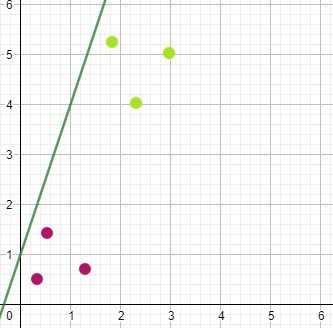
This was an awful but expected start. To improve the accuracy or, more correctly, reduce the model error, we have to calculate the value of the error. There are many ways to do this. It is not essential to understand how but it can be as simple as measuring the distance of each point from the line.
A plot on the wrong side of the line would have a high error value, and its distance will increase the error value. After calculating the error (known as a loss function), a process called Gradient Descent determines how much the line should be moved to reduce the model error and in what direction. It does so in tiny steps. The function for the new line is computed. After every training run, the error is recalculated, and adjustments continue to be made until no more improvements are seen.

The working model now allows the network to predict the label of any future item. In other words, if I input the diameter and mass of an object, the neural network can classify the object as a marble or bowling ball by using the trained function and computing which side of the line the plot from our new unlabeled data lies.
Clearly, this model sucks. I could input the diameter and mass of a tire, and the model would predict that it is a bowling ball. The model was never trained to classify tires. This is what is known as narrow AI. To be more accurate, it is not even a narrow AI. The neural network described here would never be used to solve a real-world problem.
In typical applications, the data is not as clear-cut as that in our example. With complex data, reducing the error rate to zero is impossible. Furthermore, it is not always cost-effective to aim for the lowest possible error. The energy resources, time, and money required to train a neural network are considerable, and a point of diminishing returns will be reached.
Multiple Inputs and Multiple Layers
The truth is that the simple example of separating bowling balls and marbles is nonsense. Neural networks used for simple logistic regression have no practical value. Neural networks come into their own with more complicated data sets.
Cast your mind back to the first simplified diagram of a neural network. There were many input values and many additional layers. This is what they do.
With three feature inputs, the network no longer calculates a line to separate data; it calculates a plane to separate items plotted in three dimensions.
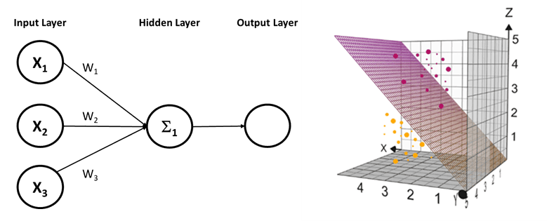
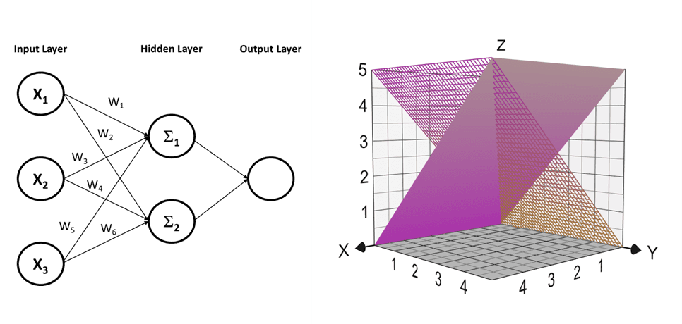
If the data cannot be separated by a single plane, we can add a second neuron to the hidden layer and create a second plane. We perform the same function twice but each time using independent weight and bias values.
Neural networks can approximate any mathematical operation, giving them the capability of separating the most complex data into groups. In this example, there are five different categories of data,
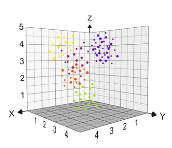
It is difficult to determine how many planes would be required to separate the groups of data from the plot effectively. However, if it were three planes, then three nodes in the hidden layer are needed. If it were four planes, then four nodes in the hidden layer, and so on.
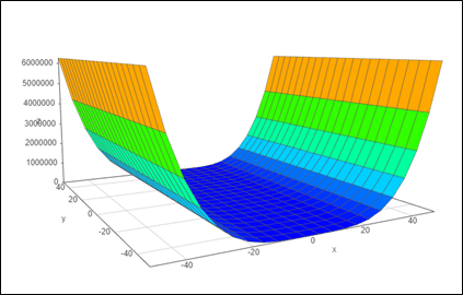
Not only can more planes be created by adding neurons to the hidden layer, but the shapes that are possible with three-dimensional functions are incredible. In all likelihood, flat planes would not work well with the previous example. Although still straightforward, a flat plane can be transformed to solve more complex challenges.
The function Z=X⁴-Y² folds the flat plane at the edges.
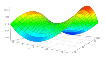
And this function increases the complexity of the plane.And
How about this?
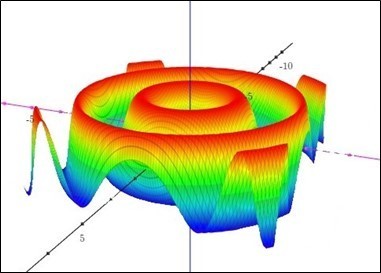
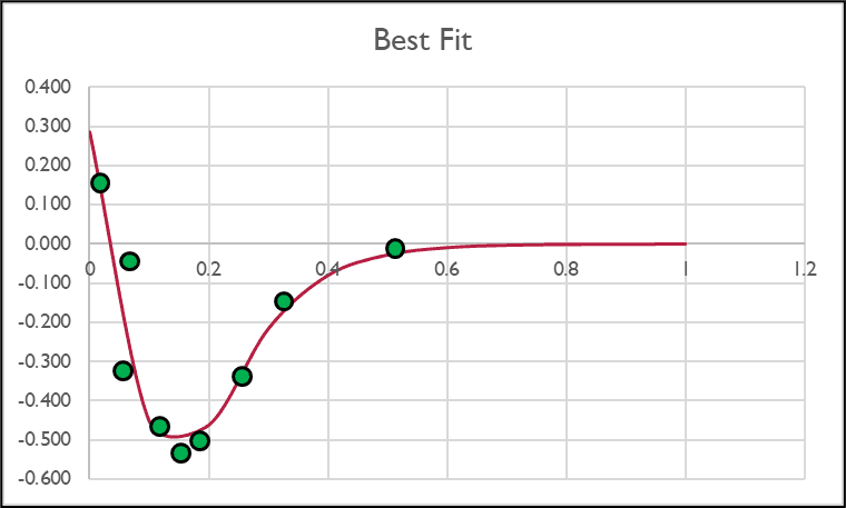
All of the functions in the examples shown require only three input features and multiple nodes in the hidden layer. However, you cannot create non-linear shapes using the linear building blocks described in this article. This is where the application of Activation Functions, mentioned earlier, comes into play. The workings of an activation function will have to wait for another article, but quite simply, they add non-linearity to a neural network. While I can’t show you a multidimensional graphic, this is an example of a math function that a neural network can approximate:
As complex as it might look, it represents this simple curved line:
The Power of Neural Networks
The example functions shown may look complicated, but to a neural network, they are not. The plots are still only three-dimensional. Imagine a four-dimensional object; for most of us, we can’t. A neural network can easily handle four dimensions; it is a simple mathematical process. Now think about a model with thousands or even millions of input features and hidden layers.
This is the power of neural networks; it takes in masses of complex data and finds valuable patterns. The latest transformer models (Think of them as a more sophisticated form of a neural network) reportedly have been trained using hundreds of billions of features and more than 1.6 trillion parameters (in straightforward terms, the weights and biases in the network). No matter how large the model is, fundamentally, they all do the same thing, separating data by creating complex shapes.
Introduction
Nobel Laureate Richard Feynman said, “When we speak without jargon, it frees us from hiding behind knowledge we don’t have. Big words and fluffy business-speak cripple us from getting to the point and passing knowledge to others.”
A grasp of the fundamentals of AI Neural networks can be useful to most business executives; however, artificial intelligence articles often require a reasonable understanding of advanced math. They invariably start by comparing neural networks and the brain’s workings. This article will explain specifically feed-forward neural networks without using either.
If you have any previous learning on AI, I am confident you have seen some form of the following diagram. It represents a small, simple, fully connected, deep neural network.

Note — A network of this small is not likely. The same outcome can be derived from simpler forms of machine learning.
But what does this network do? It simply produces mathematical functions for lines, planes, or shapes that separate or group data. That is it. That is the function of a neural network. Admittedly the shapes created by a typical neural network are multidimensional and impossible to conceptualize for all but the most brilliant people.
This example shows a plot of two things, Thing One in Purple and Thing Two in Green, and a line that separates them into groups.

A neural network is conceptually learning the mathematical function for that line. Once the network model has “learned” the math function for the line, a user can input information about a thing, i.e., the coordinates. The system will output the classification; these coordinates are to the right of the line; therefore, they represent Thing One.
A neural network connects input (features) and output (labels). Suppose I am trying to differentiate between Oranges and Bananas from features alone. The input might be the color of an object, and the output is the label Banana or Orange, both in numerical form.
The network learns the mathematical functions for lines or shapes that separate the data (this is a cat, this a dog) or fits the data (I predict this house’s price is $100k). A neural network performs multiplication, addition, and transformations to millions of numbers, each time changing its initial guess to improve the model’s accuracy. The objective of the training process is to find the numbers (called weights and biases) that result in a minor difference between the outputs of the network and the known truth.
The training process digests many examples of data relationships. The training data consists of the answer and the input features related to that answer. There are two labels in the following training data example (Car, Motorcycle) and three features (Height, Length, Weight).
Note — The choice of features here is poor and would result in a flawed AI model.
How Does it Work?
The neural network diagram in the introduction may look complicated, but it is simply a collection of smaller building blocks that look like this:

A single input feature is represented by X1. The weight is represented by W1. The strange “E” shape is the sum of the input multiplied by the weight. The B is an additional value called a Bias that is added to the previous sum. The result, called a weighted sum, is from the following mathematical function,
Weighted Sum =X1*W1+B
This is the core function of every neural network.
Note — Before being passed as an output, the weighted sum undergoes a transformation using an activation function. The activation function changes one number to another number. In simple terms, the activation function changes a linear output to a non-linear output or a straight line into a curved line.
Changing the letters from the earlier diagram and examining it more closely, you will recognize that this is the function for a straight line, i.e., Weighted Sum = X1*W1+B is the same as Y=MX+C, where M is the slope of the line and C is the slope-intercept of the Y-axis. The single neuron represents a linear function.

Now, look at this expanded neural network.

It takes two inputs instead of one, and if you examine each input individually, you will see that the resulting function is
Weighted-Sum=X1*W1+X2*W2+B
Once again, we change the letters and end up with Ax+By=C, the “Standard Form” linear function.
How Does Our Linear Function Help?
If "Thing One" represented a marble and "Thing Two" a bowling ball, a differentiation method might be to compare two features, the diameter and weight of the object. Bowling balls are larger and heavier than marbles. Before using a neural network to perform the classification task, a trained model is required.
Model Training
The training description that follows should be considered conceptual. It will give you an intuition about the workings of a neural network. If a network were to be trained using the described process, it would result in an exponential increase in the computing resources required.
Our training data will use two features that can describe bowling balls and marbles, namely diameter and mass (I am using the mass instead of weight to remove the possibility of confusion with the network parameter called weight). We naively believe that there is a mathematical function for the relationship between the diameter and the mass. This may be true, but only if the type of material used in each is identical.
The function Weighted-Sum=X1*W1+X2*W2+B is populated using random values for “W” (The weight) and “B” (The Bias). In our example, we have two weights; each could have a different value. This produces the first guess at a dividing line. We compute the weighted sum by taking the two input features, Diameter (X1) and Mass (X2), of our first object and plugging them into the function with our random weights and bias. Let’s make up some data.
W1=2, W2=3, Bias =4, Object One, Diameter = 7 and Mass=2.5
Weighted Sum = (7*2)+(2.5*3)+4, Weighted Sum = 25.5
Given Math, we know that if the features of Object One are plotted in a two-dimension graph, the point must lie on the line created by the function Weighted-Sum=X1*W1+X2*W2+B. This is perfect; we have derived the function for a line that passes through our point. In truth, any set of parameters would do the same thing for a single point. What happens when we look at the features of the second object
Object Two, Diameter=0.5 and Mass=0.1
Obviously, if we plug these into our function using the same parameters as before, the result will be different. The resulting Weighted Sum = 5.3, and unsurprisingly the second plot does not lie on the line. Given that the two feature sets represent a bowling ball and a marble, the training objective is to learn a line function that passes equidistant from both points, separating the two object classes. This is achieved by adjusting the weights and bias parameters until any errors have been eliminated.
Here three different-sized marbles in Purple and three different-sized bowling balls in Green have been plotted. The X-axis represents the diameter (input feature) of the object. The Y-axis is the known mass. When comparing the points to the calculated line, we see that all of the points lie on the same side.

This was an awful but expected start. To improve the accuracy or, more correctly, reduce the model error, we have to calculate the value of the error. There are many ways to do this. It is not essential to understand how but it can be as simple as measuring the distance of each point from the line.
A plot on the wrong side of the line would have a high error value, and its distance will increase the error value. After calculating the error (known as a loss function), a process called Gradient Descent determines how much the line should be moved to reduce the model error and in what direction. It does so in tiny steps. The function for the new line is computed. After every training run, the error is recalculated, and adjustments continue to be made until no more improvements are seen.

The working model now allows the network to predict the label of any future item. In other words, if I input the diameter and mass of an object, the neural network can classify the object as a marble or bowling ball by using the trained function and computing which side of the line the plot from our new unlabeled data lies.
Clearly, this model sucks. I could input the diameter and mass of a tire, and the model would predict that it is a bowling ball. The model was never trained to classify tires. This is what is known as narrow AI. To be more accurate, it is not even a narrow AI. The neural network described here would never be used to solve a real-world problem.
In typical applications, the data is not as clear-cut as that in our example. With complex data, reducing the error rate to zero is impossible. Furthermore, it is not always cost-effective to aim for the lowest possible error. The energy resources, time, and money required to train a neural network are considerable, and a point of diminishing returns will be reached.
Multiple Inputs and Multiple Layers
The truth is that the simple example of separating bowling balls and marbles is nonsense. Neural networks used for simple logistic regression have no practical value. Neural networks come into their own with more complicated data sets.
Cast your mind back to the first simplified diagram of a neural network. There were many input values and many additional layers. This is what they do.
With three feature inputs, the network no longer calculates a line to separate data; it calculates a plane to separate items plotted in three dimensions.

If the data cannot be separated by a single plane, we can add a second neuron to the hidden layer and create a second plane. We perform the same function twice but each time using independent weight and bias values.

Neural networks can approximate any mathematical operation, giving them the capability of separating the most complex data into groups. In this example, there are five different categories of data,

It is difficult to determine how many planes would be required to separate the groups of data from the plot effectively. However, if it were three planes, then three nodes in the hidden layer are needed. If it were four planes, then four nodes in the hidden layer, and so on.
Not only can more planes be created by adding neurons to the hidden layer, but the shapes that are possible with three-dimensional functions are incredible. In all likelihood, flat planes would not work well with the previous example. Although still straightforward, a flat plane can be transformed to solve more complex challenges.
The function Z=X⁴-Y² folds the flat plane at the edges.

And this function increases the complexity of the plane.And

How about this?

All of the functions in the examples shown require only three input features and multiple nodes in the hidden layer. However, you cannot create non-linear shapes using the linear building blocks described in this article. This is where the application of Activation Functions, mentioned earlier, comes into play. The workings of an activation function will have to wait for another article, but quite simply, they add non-linearity to a neural network. While I can’t show you a multidimensional graphic, this is an example of a math function that a neural network can approximate:
As complex as it might look, it represents this simple curved line:

The Power of Neural Networks
The example functions shown may look complicated, but to a neural network, they are not. The plots are still only three-dimensional. Imagine a four-dimensional object; for most of us, we can’t. A neural network can easily handle four dimensions; it is a simple mathematical process. Now think about a model with thousands or even millions of input features and hidden layers.
This is the power of neural networks; it takes in masses of complex data and finds valuable patterns. The latest transformer models (Think of them as a more sophisticated form of a neural network) reportedly have been trained using hundreds of billions of features and more than 1.6 trillion parameters (in straightforward terms, the weights and biases in the network). No matter how large the model is, fundamentally, they all do the same thing, separating data by creating complex shapes.
Introduction
Nobel Laureate Richard Feynman said, “When we speak without jargon, it frees us from hiding behind knowledge we don’t have. Big words and fluffy business-speak cripple us from getting to the point and passing knowledge to others.”
A grasp of the fundamentals of AI Neural networks can be useful to most business executives; however, artificial intelligence articles often require a reasonable understanding of advanced math. They invariably start by comparing neural networks and the brain’s workings. This article will explain specifically feed-forward neural networks without using either.
If you have any previous learning on AI, I am confident you have seen some form of the following diagram. It represents a small, simple, fully connected, deep neural network.

Note — A network of this small is not likely. The same outcome can be derived from simpler forms of machine learning.
But what does this network do? It simply produces mathematical functions for lines, planes, or shapes that separate or group data. That is it. That is the function of a neural network. Admittedly the shapes created by a typical neural network are multidimensional and impossible to conceptualize for all but the most brilliant people.
This example shows a plot of two things, Thing One in Purple and Thing Two in Green, and a line that separates them into groups.

A neural network is conceptually learning the mathematical function for that line. Once the network model has “learned” the math function for the line, a user can input information about a thing, i.e., the coordinates. The system will output the classification; these coordinates are to the right of the line; therefore, they represent Thing One.
A neural network connects input (features) and output (labels). Suppose I am trying to differentiate between Oranges and Bananas from features alone. The input might be the color of an object, and the output is the label Banana or Orange, both in numerical form.
The network learns the mathematical functions for lines or shapes that separate the data (this is a cat, this a dog) or fits the data (I predict this house’s price is $100k). A neural network performs multiplication, addition, and transformations to millions of numbers, each time changing its initial guess to improve the model’s accuracy. The objective of the training process is to find the numbers (called weights and biases) that result in a minor difference between the outputs of the network and the known truth.
The training process digests many examples of data relationships. The training data consists of the answer and the input features related to that answer. There are two labels in the following training data example (Car, Motorcycle) and three features (Height, Length, Weight).
Note — The choice of features here is poor and would result in a flawed AI model.
How Does it Work?
The neural network diagram in the introduction may look complicated, but it is simply a collection of smaller building blocks that look like this:

A single input feature is represented by X1. The weight is represented by W1. The strange “E” shape is the sum of the input multiplied by the weight. The B is an additional value called a Bias that is added to the previous sum. The result, called a weighted sum, is from the following mathematical function,
Weighted Sum =X1*W1+B
This is the core function of every neural network.
Note — Before being passed as an output, the weighted sum undergoes a transformation using an activation function. The activation function changes one number to another number. In simple terms, the activation function changes a linear output to a non-linear output or a straight line into a curved line.
Changing the letters from the earlier diagram and examining it more closely, you will recognize that this is the function for a straight line, i.e., Weighted Sum = X1*W1+B is the same as Y=MX+C, where M is the slope of the line and C is the slope-intercept of the Y-axis. The single neuron represents a linear function.

Now, look at this expanded neural network.

It takes two inputs instead of one, and if you examine each input individually, you will see that the resulting function is
Weighted-Sum=X1*W1+X2*W2+B
Once again, we change the letters and end up with Ax+By=C, the “Standard Form” linear function.
How Does Our Linear Function Help?
If "Thing One" represented a marble and "Thing Two" a bowling ball, a differentiation method might be to compare two features, the diameter and weight of the object. Bowling balls are larger and heavier than marbles. Before using a neural network to perform the classification task, a trained model is required.
Model Training
The training description that follows should be considered conceptual. It will give you an intuition about the workings of a neural network. If a network were to be trained using the described process, it would result in an exponential increase in the computing resources required.
Our training data will use two features that can describe bowling balls and marbles, namely diameter and mass (I am using the mass instead of weight to remove the possibility of confusion with the network parameter called weight). We naively believe that there is a mathematical function for the relationship between the diameter and the mass. This may be true, but only if the type of material used in each is identical.
The function Weighted-Sum=X1*W1+X2*W2+B is populated using random values for “W” (The weight) and “B” (The Bias). In our example, we have two weights; each could have a different value. This produces the first guess at a dividing line. We compute the weighted sum by taking the two input features, Diameter (X1) and Mass (X2), of our first object and plugging them into the function with our random weights and bias. Let’s make up some data.
W1=2, W2=3, Bias =4, Object One, Diameter = 7 and Mass=2.5
Weighted Sum = (7*2)+(2.5*3)+4, Weighted Sum = 25.5
Given Math, we know that if the features of Object One are plotted in a two-dimension graph, the point must lie on the line created by the function Weighted-Sum=X1*W1+X2*W2+B. This is perfect; we have derived the function for a line that passes through our point. In truth, any set of parameters would do the same thing for a single point. What happens when we look at the features of the second object
Object Two, Diameter=0.5 and Mass=0.1
Obviously, if we plug these into our function using the same parameters as before, the result will be different. The resulting Weighted Sum = 5.3, and unsurprisingly the second plot does not lie on the line. Given that the two feature sets represent a bowling ball and a marble, the training objective is to learn a line function that passes equidistant from both points, separating the two object classes. This is achieved by adjusting the weights and bias parameters until any errors have been eliminated.
Here three different-sized marbles in Purple and three different-sized bowling balls in Green have been plotted. The X-axis represents the diameter (input feature) of the object. The Y-axis is the known mass. When comparing the points to the calculated line, we see that all of the points lie on the same side.

This was an awful but expected start. To improve the accuracy or, more correctly, reduce the model error, we have to calculate the value of the error. There are many ways to do this. It is not essential to understand how but it can be as simple as measuring the distance of each point from the line.
A plot on the wrong side of the line would have a high error value, and its distance will increase the error value. After calculating the error (known as a loss function), a process called Gradient Descent determines how much the line should be moved to reduce the model error and in what direction. It does so in tiny steps. The function for the new line is computed. After every training run, the error is recalculated, and adjustments continue to be made until no more improvements are seen.

The working model now allows the network to predict the label of any future item. In other words, if I input the diameter and mass of an object, the neural network can classify the object as a marble or bowling ball by using the trained function and computing which side of the line the plot from our new unlabeled data lies.
Clearly, this model sucks. I could input the diameter and mass of a tire, and the model would predict that it is a bowling ball. The model was never trained to classify tires. This is what is known as narrow AI. To be more accurate, it is not even a narrow AI. The neural network described here would never be used to solve a real-world problem.
In typical applications, the data is not as clear-cut as that in our example. With complex data, reducing the error rate to zero is impossible. Furthermore, it is not always cost-effective to aim for the lowest possible error. The energy resources, time, and money required to train a neural network are considerable, and a point of diminishing returns will be reached.
Multiple Inputs and Multiple Layers
The truth is that the simple example of separating bowling balls and marbles is nonsense. Neural networks used for simple logistic regression have no practical value. Neural networks come into their own with more complicated data sets.
Cast your mind back to the first simplified diagram of a neural network. There were many input values and many additional layers. This is what they do.
With three feature inputs, the network no longer calculates a line to separate data; it calculates a plane to separate items plotted in three dimensions.

If the data cannot be separated by a single plane, we can add a second neuron to the hidden layer and create a second plane. We perform the same function twice but each time using independent weight and bias values.

Neural networks can approximate any mathematical operation, giving them the capability of separating the most complex data into groups. In this example, there are five different categories of data,

It is difficult to determine how many planes would be required to separate the groups of data from the plot effectively. However, if it were three planes, then three nodes in the hidden layer are needed. If it were four planes, then four nodes in the hidden layer, and so on.
Not only can more planes be created by adding neurons to the hidden layer, but the shapes that are possible with three-dimensional functions are incredible. In all likelihood, flat planes would not work well with the previous example. Although still straightforward, a flat plane can be transformed to solve more complex challenges.
The function Z=X⁴-Y² folds the flat plane at the edges.

And this function increases the complexity of the plane.And

How about this?

All of the functions in the examples shown require only three input features and multiple nodes in the hidden layer. However, you cannot create non-linear shapes using the linear building blocks described in this article. This is where the application of Activation Functions, mentioned earlier, comes into play. The workings of an activation function will have to wait for another article, but quite simply, they add non-linearity to a neural network. While I can’t show you a multidimensional graphic, this is an example of a math function that a neural network can approximate:
As complex as it might look, it represents this simple curved line:

The Power of Neural Networks
The example functions shown may look complicated, but to a neural network, they are not. The plots are still only three-dimensional. Imagine a four-dimensional object; for most of us, we can’t. A neural network can easily handle four dimensions; it is a simple mathematical process. Now think about a model with thousands or even millions of input features and hidden layers.
This is the power of neural networks; it takes in masses of complex data and finds valuable patterns. The latest transformer models (Think of them as a more sophisticated form of a neural network) reportedly have been trained using hundreds of billions of features and more than 1.6 trillion parameters (in straightforward terms, the weights and biases in the network). No matter how large the model is, fundamentally, they all do the same thing, separating data by creating complex shapes.

Jan 31, 2025
The Hidden Crisis in Business: When Optimization Masks a Lack of True Differentiation
When revenue stalls, leaders rush to optimize processes, trim costs, and demand more from teams. But what if the problem isn’t how well you’re executing—it’s that no one cares what you’re executing?
Jan 11, 2025
Strategy vs. Execution: Why Execution Must Come First
There’s a popular saying in business: “Vision without execution is just hallucination.” While a bit tongue-in-cheek, it captures an important lesson. Regardless of how impressive or innovative your strategy might be, if your organization can’t implement it effectively, the strategy itself is doomed.

Jan 10, 2025
From the Control Tower to the Corner Office: A Lesson in Leadership and Communication
As an air traffic controller, proactive thinking is survival. You predict weather changes, anticipate pilot error, and arrange flight paths with near-clairvoyant foresight. In corporate leadership, being proactive is equally critical. But in business, you have an entire workforce that needs to understand why you’re making the calls that you do.

Jan 31, 2025
The Hidden Crisis in Business: When Optimization Masks a Lack of True Differentiation
When revenue stalls, leaders rush to optimize processes, trim costs, and demand more from teams. But what if the problem isn’t how well you’re executing—it’s that no one cares what you’re executing?

Jan 11, 2025
Strategy vs. Execution: Why Execution Must Come First
There’s a popular saying in business: “Vision without execution is just hallucination.” While a bit tongue-in-cheek, it captures an important lesson. Regardless of how impressive or innovative your strategy might be, if your organization can’t implement it effectively, the strategy itself is doomed.

Jan 31, 2025
The Hidden Crisis in Business: When Optimization Masks a Lack of True Differentiation
When revenue stalls, leaders rush to optimize processes, trim costs, and demand more from teams. But what if the problem isn’t how well you’re executing—it’s that no one cares what you’re executing?
NeWTHISTle Consulting
DELIVERING CLARITY FROM COMPLEXITY
Copyright © 2024 NewThistle Consulting LLC. All Rights Reserved
NeWTHISTle Consulting
DELIVERING CLARITY FROM COMPLEXITY
Copyright © 2024 NewThistle Consulting LLC. All Rights Reserved
NeWTHISTle Consulting
DELIVERING CLARITY FROM COMPLEXITY
Copyright © 2024 NewThistle Consulting LLC. All Rights Reserved
